MATLAB

Introduction to MATLAB Programming

Accessing MATLAB

MATLAB can be assessed through various modes.

1. Accessing MATLAB online.

• MATLAB can be accessed online, free of charge through “mathworks” website.
• Go to https://www.mathworks.com/accesslogin/createProfile.do and create an account following the instructions.
• NOTE: Remember your Email and Password information for later use. For ‘How will you use MathWorks software?’, select “Academic use ”.

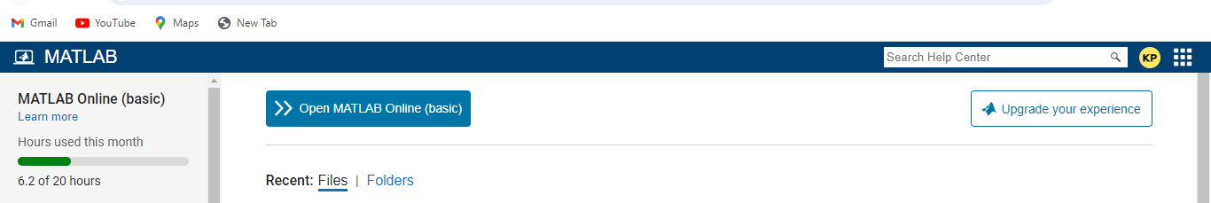
• Go to https://matlab.mathworks.com/
• Click on “open MATLAB online” and access the free version of MATLAB online. 

2. Installing Licensed version of MATLAB.

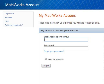
• Create a “mathworks” account.
• Login to your MathWorks account here: https://www.mathworks.com/accesslogin/login.do

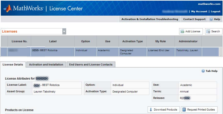
• Associate mathworks license on : https://www.mathworks.com/licensecenter
• Click on add license, when prompted add license and activation key.
• Verify association in License Center. License Label should say ‘2XXX- BEST Robotics’. (2XXX = Current Year)

• Download the Software. Go to http://www.mathworks.com/downloads/web_downloads/  🡪 Click on the Download link 🡪 Click the blue button that says R2XXXx. 🡪 Click the blue button that says R2XXXx Installer. 🡪 Open the installer file (*.exe) to extract and launch the installer.
• Install the software. When MathWorks Installer is launched, select Log in with a MathWorks Account and continue through the Installer 🡪 At the License Agreement, select Yes and continue🡪 When prompted to Log In, use your MathWorks Account info🡪 At License Selection dialog, choose ‘Select a license:’ and choose the one with the Label: 2XXX – BEST Robotics and continue.
• At the Installation Complete prompt, ensure to check Activate MATLAB (default is checked) and continue🡪 At the Confirmation dialog, click Confirm. 🡪 Activation has been completed. Click Finish.

3. Installing free MATLAB using University email address.

• Go to official website of University of Delhi 🡪 Libraries 🡪 e-Resources 🡪 scroll down 🡪IT service 🡪”Get Software” in the list on the left-hand side 🡪 MATLAB 🡪Create an account using university email address and install licensed version of MATLAB.
• Alternately, go to https://in.mathworks.com/academia/tah-portal/university-of-delhi-40795990.html and create an account using email Id provided be the university and install MATLAB.

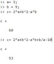
Basics: Variables and Operators

1. Defining Variables: 

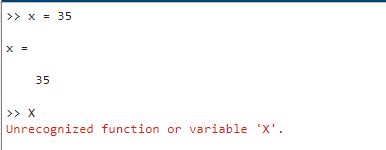
• MATLAB variables are case sensitive which means “x” and “X” can be used as different variables and store different values.

• Variables names can have up to 63 characters (MATLAB 6.5 or newer)
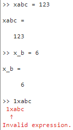
• Variable names can start with a letter and can be followed by digits or underscores.

2. Special Variables: 

• Inf = infinity
• NaN = Not a number
• eps = smallest possible incremental Value 
• pi 
• i and j = root of -1
• realmin = smallest usable positive real number
• realmax = largest usable positive real number

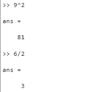
Operators in MATLAB:

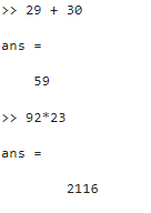
1. Arithmetic operators 

1	Add	a+b
2	Subtract	a-b
3	Multiply	a*b
4	Divide	a/b
5	Exponent	a^b

2. Relational operators

1	Greater than	>
2	Less than	<
3	Greater than or equal to	>=
4	Less than or equal to	<=
5	Equal to	==
6	Not Equal to	~=

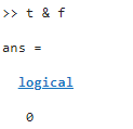
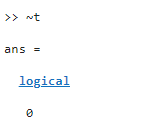
3. Logical operators 

1	~	NOT
2	&	AND
3	|	OR

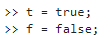
Note: The semicolon “;” after the statements suppresses the output

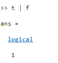
Note : “NOT” operator has the highest precendence and “AND” and “OR” lie on the same precendence level.

Elementary Mathematical functions:

• abs – finds absolute value of all elements in the matrix.
• sign – signum function.
• sin, cos – Trigonometric functions.
• asin, acos… – Inverse trigonometric functions. 
• exp – Exponential. 
• Log, log10 – natural logarithm, logarithm (base 10) 
•  ceil, floor – round towards +infinity, -infinity respectively.
• round – round towards nearest integer. 
•  real, imag – real and imaginary part of a complex matrix.
• sort – sort elements in ascending order.

Matrices

• A matrix can be created as follows (carefully observe the position of comas and semicolons) 

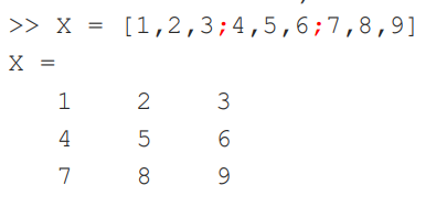
• In MATLAB indexing starts from 1.
• Each element can be accessed from the matrix using the indices of its row and column in the same order.
• For example: “2” can be accessed as X(1,2) 

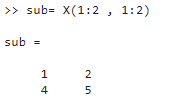
• A portion of a matrix can be extracted into another variable using the following syntax :

                       Submatrix = Matrix(r1:r2 , c1:c2 )

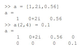
Manipulating Matrices:

1. Matrix extension 

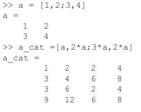
2. Concatenation

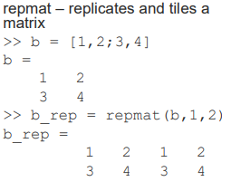
3. Repetition 

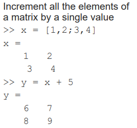
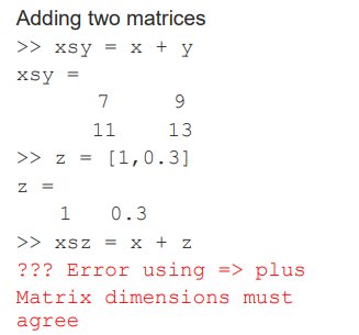
4. Addition 

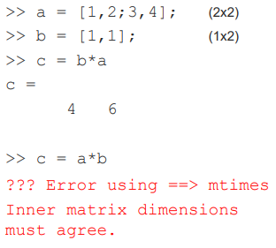
5. Matrix multiplication

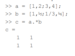
Element wise multiplication:

MATLAB matrices Functions:

• zeros: creates an array of all zeros, Ex: x = zeros(3,2). 
• ones: creates an array of all ones, Ex: x = ones(2).  
• eye: creates an identity matrix, Ex: x = eye(3). 
• rand: generates uniformly distributed random numbers in [0,1].
• diag: Diagonal matrices and diagonal of a matrix.
• size: returns array dimensions.
• length: returns length of a vector (row or column).
• det: Matrix determinant.
• inv: matrix inverse.
• eig: evaluates eigenvalues and eigenvectors.
• rank: rank of a matrix 
• find: searches for the given values in an array/matrix.

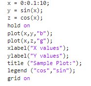
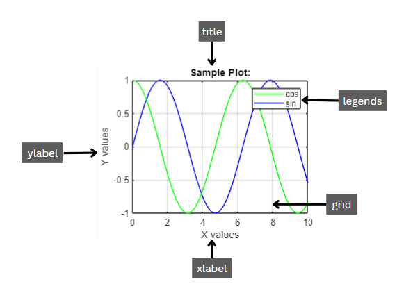
2D Plotting:

Different Function that are used for plotting graphs: 

1	plot(x,y)	Plot a continuous graph between x and y.
2	stem(x,y)	Plotting a discrete graph between x and y.
3	Legends(“text1”, “text2”)	Used to tell what a graph represents.
4	title(“text”)	Used to give a title to the graph.
5	xlabel(“text”)	Label X-axis.
6	ylabel(“text”)	Label Y-axis.
7	figure	Creating a new container figure on which the graph is plotted
8	grid on	To create a grid on the figure.
10	subplot(a, b, p)	To view different plots on different sub-figures simultaneously on a grid view. (a is number of rows of the grid, b is the number of columns and p indicates the position of the plot in the grid)

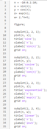
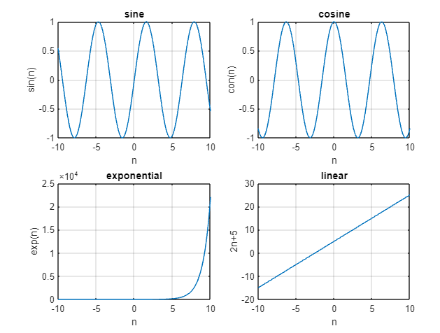
Example: 

Use of subplot:

Subplot is used to create multiple plots on same window in a grid format. Subplot is used with the syntax: subplot(R,C,I). Where “R” is the total number of rows of the grid, “C” is the total number of columns of the grid and “I” indicates the index of the plot on the grid

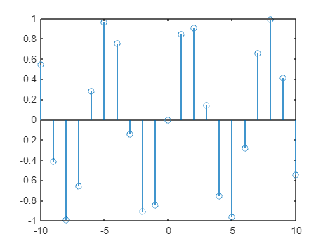
Use of “stem”:

“stem” is used to plot a signal or a graph where x axis is discretised.

Example:

Flow of control:

MATLAB has 5 flow control statements:

1. “if”/ “else” statement
2. “switch” statement.
3. “for” loops.
4. “while” loops.
5. “break” statement.

All these statements form a block that start with the head of the statement and end with with “end” in the following syntax:

if condition

:

:

:

end

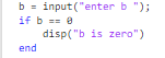
If statement:

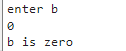
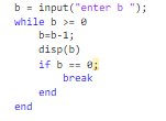
“while” Loops with “break” statement

• While loop, runs a command or a set of command repeatedly until the given condition becomes false.
• There is an update statement within the loop, that updates the condition, and then decides when the flow of control exits the loop.
• “break” statement can be used to break a “for” or “while” loop.

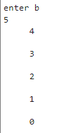
“for” loops

• For loop repeats a command or a set of commands a specific number of times.
• It assigns and overrides the value of an iterating variables from a specified range and the flow of control exits the loop, when there is no value remains in the given range to be assigned to the variable.

Simulink:

Simulink is a block diagram environment used to design systems with multidomain models, simulate before moving to hardware, and deploy without writing code.

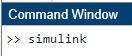
Starting Simulink:

To start simulink write in command window : simulink and press enter.

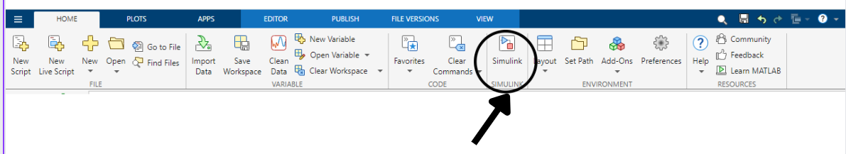
Alternatively, you can click on simulink button on the toolbar.

This is what the simulink start page looks like:

Click on blank Model create a blank workspace.

Go to library browser to explore multiple toolboxes. Each toolbox contains multiple corresponding blocks that can be used to create a block diagram and run simulation.

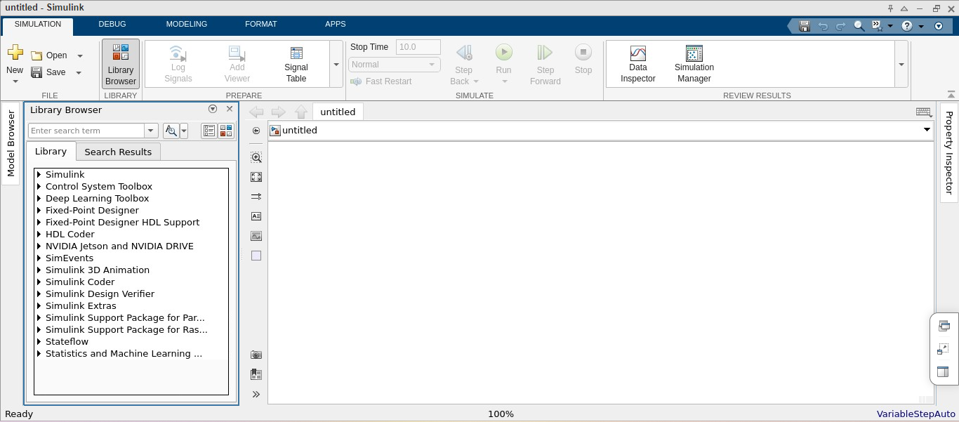
Under “simulink” you can find multiple classes of blocks:

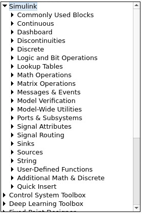
Some of them are used as follows:

• Sources: Used to generate various signals.

• Sinks: Used to output or display signals. 

• Discrete: Linear, discrete-time system elements (transfer functions, state-space models, etc.).

• Linear: Linear, continuous-time system elements and connections (summing junctions, gains, etc.). 

• Nonlinear: Nonlinear operators (arbitrary functions, saturation, delay, etc.). 

• Connections: Multiplex, Demultiplex, System Macros, etc. 

Blocks have zero to several input terminals and zero to several output terminals. Unused input terminals are indicated by a small open triangle. Unused output terminals are indicated by a small triangular point. The block shown below has an unused input terminal on the left and an unused output terminal on the right.

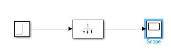
Simple example

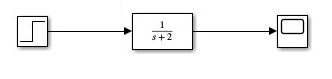
Passing a unit step signal “u(t)” through a block of a given transfer function “1/(s+1)” and observing its output using scope. 

Block diagram on simulink:

Mathematically:

• Laplace transform of u(t) is 1/s.
• When this function is given as an input of a block of impulse response h(t)=e^-t. In “s” domain this transfer function is given by 1/(s+1).
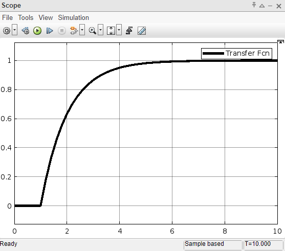
• Output of this should theoretically by the convolution integral of u(t) and h(t) or inverse Laplace transform of product of 1/s and 1/(s+1).
• Output= x(t)*h(t) = u(t)*e^-t = L ^–(1/s(s+1)) = 1-e^-t

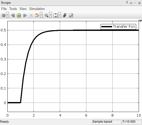
Output plot on simulink scope:

Modifying Block:

A block can be modified by double-clicking on it. if you double-click on the “Transfer Fcn” block in the example model, you will see the following dialog box.

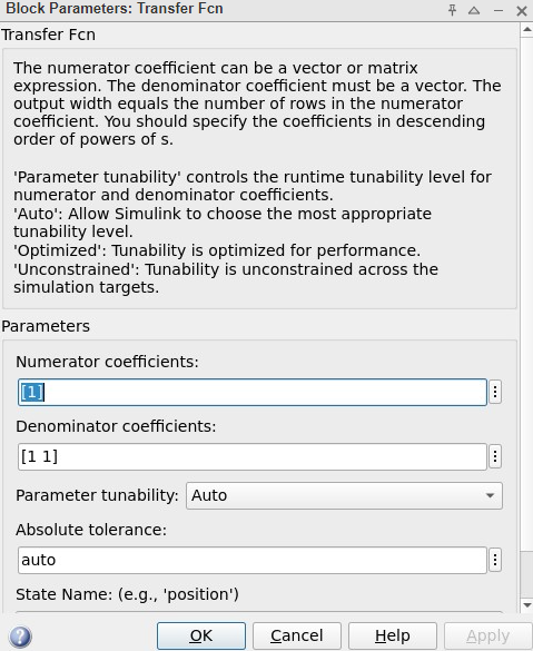
Blocks can be modified by changing the coefficient and then clicking apply:

Reference Links

1. https://www.tutorialspoint.com/matlab/index.htm
2. https://in.mathworks.com/help/matlab/getting-started-with-matlab.html
3. https://www.mccormick.northwestern.edu/documents/students/undergraduate/introduction-to-matlab.pdf